Selection Sort

Selection Sort is a simple sorting algorithm that works by repeatedly finding the minimum element from the unsorted part of the array and putting it at the beginning. The algorithm divides the array into a sorted and an unsorted region. In each iteration, it finds the minimum element in the unsorted region and swaps it with the first element of the unsorted region.

Example with Sample Data:

Let's say we have an array: [64, 25, 12, 22, 11]

1. Initial state: [64, 25, 12, 22, 11]

2. Find the minimum element in the unsorted region (11) and swap it with the first element. Array becomes [11, 25, 12, 22, 64].

3. Move the boundary between the sorted and unsorted regions.

4. Find the minimum element in the unsorted region (12) and swap it with the first element of the unsorted region. Array becomes [11, 12, 25, 22, 64].

5. Move the boundary again.

6. Continue this process until the array is sorted.

Pseudocode:

procedure selectionSort(arr: array of Comparable)
    n = length(arr)

    for i from 0 to n - 1
        // Find the minimum element in the unsorted part
        minIndex = i
        for j from i + 1 to n
            if arr[j] < arr[minIndex]
                minIndex = j

        // Swap the found minimum element with the first element
        swap(arr[i], arr[minIndex])
    end for
end procedure

Java Implementation:

public class SelectionSort {

    public static void main(String[] args) {
        int[] arr = {64, 25, 12, 22, 11};
        selectionSort(arr);
        System.out.println("Sorted array:");
        printArray(arr);
    }

    public static void selectionSort(int[] arr) {
        int n = arr.length;

        for (int i = 0; i < n - 1; i++) {
            // Find the minimum element in the unsorted part
            int minIndex = i;
            for (int j = i + 1; j < n; j++) {
                if (arr[j] < arr[minIndex]) {
                    minIndex = j;
                }
            }

            // Swap the found minimum element with the first element
            int temp = arr[minIndex];
            arr[minIndex] = arr[i];
            arr[i] = temp;
        }
    }

    public static void printArray(int[] arr) {
        for (int i = 0; i < arr.length; i++) {
            System.out.print(arr[i] + " ");
        }
        System.out.println();
    }
}

Complexity Analysis:

• Time Complexity:

  • Best Case: O(n^2) - always.

  • Average Case: O(n^2) - always.

  • Worst Case: O(n^2) - always.

• Space Complexity:

  • Selection Sort is an in-place sorting algorithm, so its space complexity is O(1).

Selection Sort has a quadratic time complexity, and like Bubble Sort, it's not recommended for large datasets. However, it has the advantage of requiring only a constant amount of additional memory space.

Bubble Sort

Bubble Sort is a simple sorting algorithm that repeatedly steps through the list, compares adjacent elements, and swaps them if they are in the wrong order. The pass through the list is repeated until the list is sorted. The name "Bubble Sort" is derived from the way smaller elements "bubble" to the top of the list.

Example with Sample Data:

Let's say we have an array: [5, 3, 8, 4, 2]

1. First Pass:

   • Compare 5 and 3. Swap because 3 < 5. Array becomes [3, 5, 8, 4, 2].

   • Compare 5 and 8. No swap because 8 > 5. Array remains [3, 5, 8, 4, 2].

   • Compare 8 and 4. Swap because 4 < 8. Array becomes [3, 5, 4, 8, 2].

   • Compare 8 and 2. Swap because 2 < 8. Array becomes [3, 5, 4, 2, 8].

After the first pass, the largest element (8) has bubbled to the end.

1. Second Pass:

   • Continue the process, but ignore the last element (8) since it's already in the correct position.

   • The array becomes [3, 4, 2, 5, 8].

2. Third Pass:

   • The array becomes [3, 2, 4, 5, 8].

3. Fourth Pass:

   • The array becomes [2, 3, 4, 5, 8].

Now, the array is sorted.

Pseudocode:

procedure bubbleSort(arr: array of Comparable)
    n = length(arr)
    for i from 0 to n - 1
        for j from 0 to n - i - 1
            // Compare adjacent elements
            if arr[j] > arr[j + 1]
                // Swap if they are in the wrong order
                swap(arr[j], arr[j + 1])
        end for
    end for
end procedure

Java Implementation:

public class BubbleSort {

    public static void main(String[] args) {
        int[] arr = {5, 3, 8, 4, 2};
        bubbleSort(arr);
        System.out.println("Sorted array:");
        printArray(arr);
    }

    public static void bubbleSort(int[] arr) {
        int n = arr.length;

        for (int i = 0; i < n - 1; i++) {
            boolean didSwap = false;
            for (int j = 0; j < n - i - 1; j++) {
                // Compare adjacent elements
                if (arr[j] > arr[j + 1]) {
                    // Swap if they are in the wrong order
                    didSwap = true;
                    int temp = arr[j];
                    arr[j] = arr[j + 1];
                    arr[j + 1] = temp;
                }
                // best case when array is already sorted
                if (didSwap) break;
            }
        }
    }

    public static void printArray(int[] arr) {
        for (int i = 0; i < arr.length; i++) {
            System.out.print(arr[i] + " ");
        }
        System.out.println();
    }
}

Complexity Analysis:

• Time Complexity:

  • Best Case: O(n) - when the array is already sorted.

  • Average Case: O(n^2) - in most cases.

  • Worst Case: O(n^2) - when the array is sorted in reverse order.

• Space Complexity:

  • Bubble Sort is an in-place sorting algorithm, so its space complexity is O(1).

Bubble Sort is generally not recommended for large datasets due to its quadratic time complexity, but it is easy to understand and implement.

Insertion Sort

Insertion Sort is a simple sorting algorithm that builds the final sorted array one item at a time. It is much less efficient on large lists than more advanced algorithms such as quicksort, heapsort, or merge sort. However, it provides several advantages: simple implementation, efficient for small datasets, and works well for partially sorted datasets.

Example with Sample Data:

Let's say we have an array: [12, 11, 13, 5, 6].

1. Initial state: [12, 11, 13, 5, 6].

2. Start with the second element (11). Compare it with the first element (12) and swap if necessary. Array becomes [11, 12, 13, 5, 6].

3. Move to the third element (13). Compare it with the previous elements and swap if necessary. Array becomes [11, 12, 13, 5, 6].

4. Continue this process for the remaining elements.

Pseudocode:

procedure insertionSort(arr: array of Comparable)
    n = length(arr)

    for i from 1 to n - 1
        current = arr[i]
        j = i - 1

        // Move elements of arr[0..i-1] that are greater than current,
        // to one position ahead of their current position
        while j >= 0 and arr[j] > current 
            arr[j + 1] = arr[j]
            j = j - 1

        // insert current element to actual position
        arr[j + 1] = current 
    end for
end procedure

Java Implementation:

public class InsertionSort {

    public static void main(String[] args) {
        int[] arr = {12, 11, 13, 5, 6};
        insertionSort(arr);
        System.out.println("Sorted array:");
        printArray(arr);
    }

    public static void insertionSort(int[] arr) {
        int n = arr.length;

        for (int i = 1; i < n; ++i) {
            int current = arr[i];
            int j = i - 1;

            // keep swapping previous elements if needed 
            while (j >= 0 && arr[j] > current) {
                arr[j + 1] = arr[j];
                j = j - 1;
            }

            // insert current element to actual position
            arr[j + 1] = current;
        }
    }

    public static void printArray(int[] arr) {
        for (int i = 0; i < arr.length; i++) {
            System.out.print(arr[i] + " ");
        }
        System.out.println();
    }
}

Complexity Analysis:

• Time Complexity:

  • Best Case: O(n) - when the array is already sorted.

  • Average Case: O(n^2) - in most cases.

  • Worst Case: O(n^2) - when the array is sorted in reverse order.

• Space Complexity:

  • Insertion Sort is an in-place sorting algorithm, so its space complexity is O(1).

Insertion Sort is efficient for small datasets and works well with partially sorted data. It is stable and adaptive, making it a good choice for certain scenarios.

Merge Sort

Merge Sort is a divide-and-conquer algorithm that works by dividing the array into two halves, recursively sorting each half, and then merging the sorted halves to produce a single sorted array. It's known for its stability and is often used for sorting linked lists.

Example with Sample Data:

Let's say we have an array: [38, 27, 43, 3, 9, 82, 10].

1. Divide the array into two halves: [38, 27, 43] and [3, 9, 82, 10].

2. Recursively apply Merge Sort to each half:

   • For the first half, [38, 27, 43], divide into [38], [27], and [43], then merge them in sorted order to get [27, 38, 43].

   • For the second half, [3, 9, 82, 10], divide into [3, 9] and [82, 10], then merge them in sorted order to get [3, 9, 10, 82].

3. Merge the two sorted halves [27, 38, 43] and [3, 9, 10, 82] to get the final sorted array [3, 9, 10, 27, 38, 43, 82].

Pseudocode:

procedure mergeSort(arr: array of Comparable)
    if length(arr) <= 1
        // Already sorted
        return

    mid = length(arr) / 2

    // Divide the array into two halves
    left = slice(arr, 0, mid)
    right = slice(arr, mid, length(arr))

    // Recursively sort the left and right halves
    mergeSort(left)
    mergeSort(right)

    // Merge the sorted left and right halves
    merge(arr, left, right)
end procedure


procedure merge(arr: array of Comparable, left: array of Comparable, right: array of Comparable)
    i = 0
    j = 0
    k = 0

    // Compare elements from the left and right arrays and merge them into the original array
    while i < length(left) and j < length(right)
        if left[i] <= right[j]
            arr[k] = left[i]
            i = i + 1
        else
            arr[k] = right[j]
            j = j + 1

        k = k + 1

    // Copy the remaining elements from the left and right arrays, if any
    while i < length(left)
        arr[k] = left[i]
        i = i + 1
        k = k + 1

    while j < length(right)
        arr[k] = right[j]
        j = j + 1
        k = k + 1
end procedure

Java Implementation:

public class MergeSort {

    public static void main(String[] args) {
        int[] arr = {38, 27, 43, 3, 9, 82, 10};
        mergeSort(arr);
        System.out.println("Sorted array:");
        printArray(arr);
    }

    public static void mergeSort(int[] arr) {
        if (arr.length <= 1) {
            return;
        }

        int mid = arr.length / 2;
        int[] left = new int[mid];
        int[] right = new int[arr.length - mid];

        System.arraycopy(arr, 0, left, 0, left.length);
        System.arraycopy(arr, mid, right, 0, right.length);

        mergeSort(left);
        mergeSort(right);

        merge(arr, left, right);
    }

    public static void merge(int[] arr, int[] left, int[] right) {
        int i = 0, j = 0, k = 0;

        while (i < left.length && j < right.length) {
            if (left[i] <= right[j]) {
                arr[k++] = left[i++];
            } else {
                arr[k++] = right[j++];
            }
        }

        // Copy the remaining elements of left and right (if any)
        while (i < left.length) {
            arr[k++] = left[i++];
        }

        while (j < right.length) {
            arr[k++] = right[j++];
        }
    }

    public static void printArray(int[] arr) {
        for (int i = 0; i < arr.length; i++) {
            System.out.print(arr[i] + " ");
        }
        System.out.println();
    }
}

Complexity Analysis:

• Time Complexity:

  • Best Case: O(n log n) - always.

  • Average Case: O(n log n) - always.

  • Worst Case: O(n log n) - always.

• Space Complexity:

  • Merge Sort has a space complexity of O(n) due to the additional space required for the temporary arrays during the merging step.

Quick Sort

QuickSort is a divide-and-conquer algorithm that works by selecting a 'pivot' element from the array and partitioning the other elements into two sub-arrays according to whether they are less than or greater than the pivot. The sub-arrays are then sorted recursively.

Example with Sample Data:

Let's say we have an array: [38, 27, 43, 3, 9, 82, 10].

1. Choose a pivot, for example, 27.

2. Partition the array into two sub-arrays:

   • Elements less than the pivot: [3, 9, 10]

   • Elements greater than the pivot: [38, 27, 43, 82]

3. Recursively apply QuickSort to each sub-array.

4. After sorting the sub-arrays, concatenate them with the pivot in the middle: [3, 9, 10, 27, 38, 43, 82].

Pseudocode:

procedure quickSort(arr: array of Comparable, low: int, high: int)
    if low < high
        pivotIndex = partition(arr, low, high)
        quickSort(arr, low, pivotIndex - 1)
        quickSort(arr, pivotIndex + 1, high)

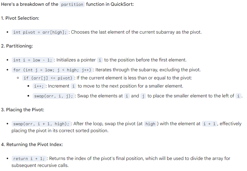
procedure partition(arr: array of Comparable, low: int, high: int) -> int
    pivot = arr[high]
    i = low - 1

    for j from low to high - 1
        if arr[j] <= pivot
            i = i + 1
            swap(arr[i], arr[j])

    swap(arr[i + 1], arr[high])
    return i + 1

Java Implementation:

public class QuickSort {

    public static void main(String[] args) {
        int[] arr = {38, 27, 43, 3, 9, 82, 10};
        quickSort(arr, 0, arr.length - 1);
        System.out.println("Sorted array:");
        printArray(arr);
    }

    public static void quickSort(int[] arr, int low, int high) {
        if (low < high) {
            int pivotIndex = partition(arr, low, high);
            quickSort(arr, low, pivotIndex - 1);
            quickSort(arr, pivotIndex + 1, high);
        }
    }

    public static int partition(int[] arr, int low, int high) {
        int pivot = arr[high];
        int i = low - 1;

        for (int j = low; j < high; j++) {
            if (arr[j] <= pivot) {
                i++;
                swap(arr, i, j);
            }
        }

        swap(arr, i + 1, high);
        return i + 1;
    }

    public static void swap(int[] arr, int i, int j) {
        int temp = arr[i];
        arr[i] = arr[j];
        arr[j] = temp;
    }

    public static void printArray(int[] arr) {
        for (int i = 0; i < arr.length; i++) {
            System.out.print(arr[i] + " ");
        }
        System.out.println();
    }
}

Complexity Analysis:

• Time Complexity:

  • Best Case: O(n log n) - when the partitioning is well-balanced.

  • Average Case: O(n log n) - on average.

  • Worst Case: O(n^2) - occurs when the pivot selection consistently results in an unbalanced partitioning.

• Space Complexity:

  • QuickSort is an in-place sorting algorithm, so its space complexity is O(1).